多元线性回归

推导

在广义的线性回归中，是可以有多个变量或者多个特征的，在上一篇文章线性回归算法中实现了一元线性回归，但在实际问题当中，决定一个label经常是由多个变量或者特征决定的。在一元线性回归当中，问题最终转化为使得误差函数最小的$a$和$b$，预测函数为$\hat{y}^{(i)}=ax^{(i)}+b$，也可以写成这种形式$\hat{y}=\theta_0+\theta_1x$，其中$\theta_0$为截距$b$，$\theta_1$为前面式子中的$a$

那么对于在多元线性回归，我们也可以将预测函数函数表示为

问题转化为求满足上述预测函数且误差函数最小的

令$X_0^{(i)}\equiv1$,则有

其中

所以预测函数可以写成是$\hat{y}^{(i)}=X^{(i)}\cdot \theta$，对于这个预测函数，要使得损失函数$\sum\limits_{i=1}^m(y^{(i)}-\hat{y}^{(i)})^2$尽可能小，经过推导可以得到等价于使得$(y-X_b\cdot\theta)^T(y-X_b\cdot\theta)$尽可能小，则有$\theta$的正规方程解(Normal Equation)：

但是这种方法存在缺点，即计算的时间复杂度比较高，为$O(n^3)$，即便经过优化后可以达到$O(n^{2.4})$，但还是效率比较低。这种方法也有优点，那就是不用对数据做归一化处理。

对于得到的$\theta=(\theta_0,\theta_1,\theta_2,…，\theta_n)^T$中，$\theta_0$为截距(intercept)，$\theta_1,\theta_2,…，\theta_n$为系数(coefficients)

实现

多元线性回归

# 读取波士顿房价数据
boston = datasets.load_boston()
x=boston.data
y=boston.target

# 去除边界点
x = x[y<50.0]
y = y[y<50.0]
x.shape
# (490, 13)
# 可以看到具有13个变量/特征值

from sklearn.model_selection import train_test_split
from sklearn.linear_model import LinearRegression

x_train,x_test,y_train,y_test = train_test_split(x,y,random_state = 666)
lin_reg = LinearRegression()
lin_reg.fit(x_train,y_train)
# LinearRegression(copy_X=True, fit_intercept=True, n_jobs=None, normalize=False)

# 参数
lin_reg.coef_
# array([-1.15625837e-01,  3.13179564e-02, -4.35662825e-02, -9.73281610e-02,
#       -1.09500653e+01,  3.49898935e+00, -1.41780625e-02, -1.06249020e+00,
#        2.46031503e-01, -1.23291876e-02, -8.79440522e-01,  8.31653623e-03,
#       -3.98593455e-01])

# 截距
lin_reg.intercept_
# 32.59756158869959

# 评分
lin_reg.score(x_test,y_test)
# 0.8009390227581041

kNN回归

from sklearn.neighbors import KNeighborsRegressor

knn_reg = KNeighborsRegressor()
knn_reg.fit(x_train,y_train)

# KNeighborsRegressor(algorithm='auto', leaf_size=30, metric='minkowski',
#                    metric_params=None, n_jobs=None, n_neighbors=5, p=2,
#                    weights='uniform')

knn_reg.score(x_test,y_test)
# 0.602674505080953


# 使用网格搜索寻找最优参数
from sklearn.model_selection import GridSearchCV
# 定义网格
param_grid=[
    {
        'weights':['uniform'],
        "n_neighbors":[i for i in range(1,11)]
    },
    {
        'weights':['distance'],
        'n_neighbors':[i for i in range(1,11)],
        'p':[i for i in range(1,6)]
    }
]

knn_reg = KNeighborsRegressor()
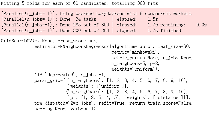
grid_search = GridSearchCV(knn_reg, param_grid,n_jobs = -1,verbose = 1)
grid_search.fit(x_train,y_train)
# 运行结果如下图

grid_search.best_params_
# {'n_neighbors': 6, 'p': 1, 'weights': 'distance'}
grid_search.best_score_
# 0.6243135119018297
# 这个分数是使用交叉验证得到的分数，不是上面的R square方法得到的

grid_search.best_estimator_.score(x_test,y_test)
# 0.7353138117643773